機器有辦法自行從文本中觀察出詞彙間的相似度嗎?是可以的,word2vec是"word to vector"的縮寫,代表的正是將每個字轉換成向量,而一旦兩個字的向量越是靠近,就代表它的相似度越高,我們究竟要如何得到這些向量呢?方法簡單但出奇有效,文章的最後會向大家呈現它的精彩的結果。
本單元程式碼Skip-Gram Word2Vec部分可於Github下載,CBOW Word2Vec部分可於Github下載。
Word2Vec觀念解析
Word2Vec的形式和Autoencoder有點像,一樣是從高維度的空間轉換到低維度的空間,再轉換回去原本的維度,只是這一次轉回去的東西不再是原本一模一樣的東西了。
Word2Vec的Input和Output這次變成是上下文的文字組合,舉個例子,"by the way"這個用法如果多次被機器看過的話,機器是有辦法去學習到這樣的規律的,此時"by"與"the"和"way"便會產生一個上下文的關聯性,為了將這樣的關聯性建立起來,我們希望當我輸入"by"時,機器有辦法預測並輸出"the"或"way",這代表在機器內部它已經學習到了上下文的關聯性。
那如果今天這個機器也同時看到很多次的"on the way"這種用法,所以當我輸入"on"時,機器要有辦法預測並輸出"the"或"way",但是我們不希望"on"和"by"兩個詞在學習時是分開學習的,我們希望機器可以因為"by the way"和"on the way"的結構很相似,所以有辦法抓出"on"和"by"是彼此相似的結論。
如何做到呢?答案就是限縮這個上下文的關聯性的儲存維度,如果我的字彙量有1000個,這1000個字彙彼此有上下文的關聯性,最完整表示上下文關聯性的方法就是設置一個1000x1000或者更大的表格,把所有字彙間的上下文關聯性全部存起來,但我們不想要這麼做,我要求機器用更小的表格來儲存上下文的關聯性,此時機器被迫將一些詞彙使用同樣的表格位置,同樣的轉換。一旦限縮了上下文關聯性的儲存維度,"on the way"和"by the way"中的"on"和"by"就會被迫分為同一類,因此我們成功的建立了字詞間的相似性關係。
Word2Vec的架構
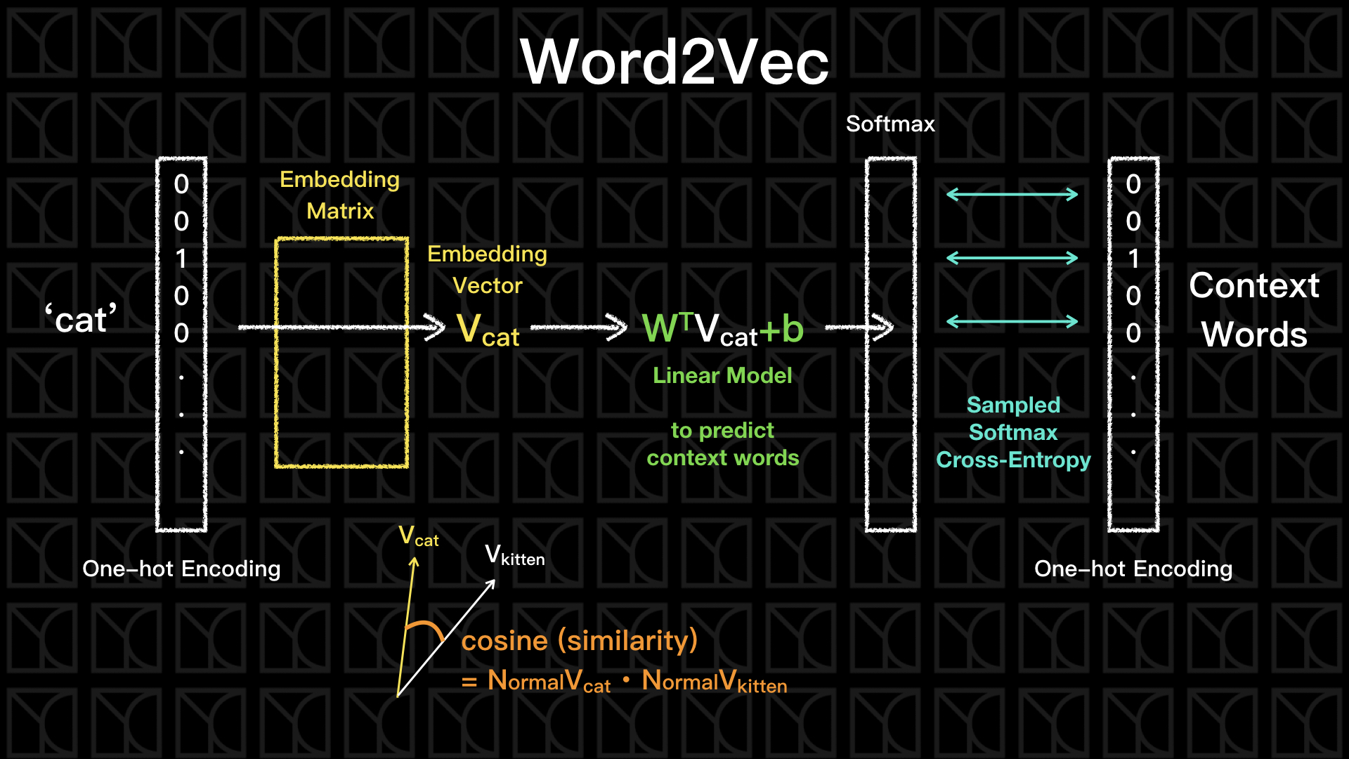
實作上如上圖所示,我們輸入一個字詞,譬如"cat",通常會將他轉成One-hot encoding表示,但要注意喔!文本的字彙量是非常龐大的,所以當我們使用One-hot encoding表示時,將會出現一個非常長但Sparse的向量,相同的輸出層也同樣是一個很長的One-hot encoding,它的維度會和輸入層一樣大,因為我們要分析的字彙在輸入和輸出是一樣多的。
然後,和Autoencoder使用一樣的手法,中間的Hidden Layer放置低維度、少神經元的一層,但不同於Autoencoder,Word2Vec所有的轉換都是線性的,沒有非線性的Activation Function夾在其中,為什麼呢?因為我們的輸入是Sparse的而且只有0和1的差別,所以每一條通路就變成只有導通或不導通的差別,Activation Function有加等於沒加,使用線性就足夠了。
這個中間的Hidden Layer被稱為Embedding Matrix,它做了一個線性的Dimension Reduction,將原本高維度的One-hot encoding降低成低維度,然後再透過一個線性模型轉換回去原本的維度。假設字彙的數量有N個,所以輸入矩陣X是一個1xN的矩陣,輸出的矩陣同樣也是1xN的矩陣,當我先做一個線性的Dimension Reduction,將維度降到d維,此時Embedding Matrix會是一個Nxd的矩陣V,然後再由線性模型轉換回去原本的維度,這個轉換矩陣W是一個Nxd矩陣,因此綜合上述,可用一個簡潔的表示式表示:\(Y=W^T VX\),我們的目標就是找出這個W和V矩陣的每個元素。
你會想說線性模型很簡單啊!就是仿照Autoencoder的作法,然後把Activation Function拿掉不就了事了,並且因為輸出是One-hot Encoding所以最後套用Softmax,那不就輕鬆完成!但是真正的大魔王就出在字彙量,字彙量一旦很大,事情就變得不可收拾了,而且字彙量是一定小不得的,那怎麼辦?
在Dimension Reduction我們可以採取一個快速的方法,因為除了我要表示的字的位置是1以外其他都是0,所以其他都可以不看,我們就直接看是在第幾個位置上是1,然後再到Embedding Matrix上找到相應的行直接取出就是答案了,這樣查詢的動作,在Tensorflow中可以使用tf.nn.embedding_lookup來辦到。
再接下來最後的Cross-Entropy Loss計算也非常龐大,因為有幾個字彙就需要累加幾組數字,我們有一招偷吃步的方法叫做「Sampled Softmax」,作法是這樣的,我們不去計算全部詞彙的Cross-Entropy,而是選擇幾組詞彙來評估Cross-Entropy,在選擇上我們會隨機挑選一些Labels和預測結果差異度很大的詞彙(稱為Negative Examples)來算Cross-Entropy,我們在Tensorflow可以使用tf.nn.sampled_softmax_loss來辦到「Sampled Softmax」。
我們先不管輸入和輸出究竟怎麼取得,如果我們成功的建立了輸入和輸出的上下文關係,此時中間的Embedding空間正是精華的所在,經過剛剛推論,我們預期在這個空間當中,相似的詞彙會彼此靠近,我們評估兩個向量的相似性可以使用Cosine來評估,當兩向量的夾角越小代表它們越是相似,待會的實作當中我們將會利用Cosine來建立Similarity的大小,藉此來找到前幾個和它很靠近的詞彙。
另外,經研究指出這個Embedding空間的效果不只是可以算出詞彙間的相似性,還可以顯示詞彙間的比較關係,例如:北京之於中國,等同於台北之於台灣,這樣的比較關係也顯示在這個Embedding空間裡頭,所以在這空間裡會有以下的向量關係式:\(V_{北京} - V_{中國}+V_{台灣}=V_{台北}\),是不是很神奇啊!
Word2Vec的兩種常用方法:Skip-Gram和CBOW
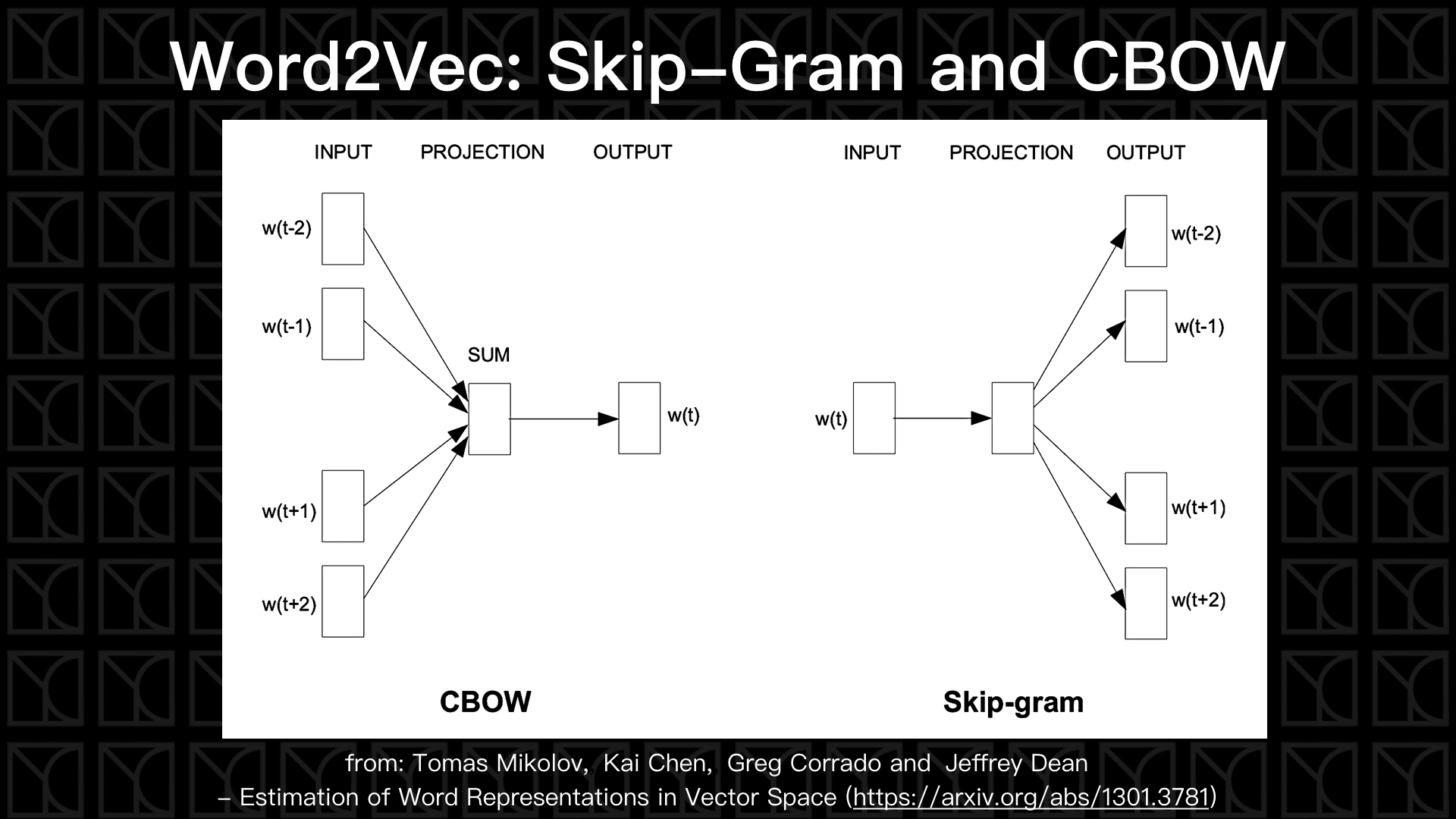
剛剛一直在講的是中間的結構應該怎麼建立,現在來看看我們可以輸入和輸出哪些詞彙來建立起上下文的關係,有兩種常用的類別:Skip-Gram和CBOW。
Skip-Gram如上圖所示,當我輸入一個\(word(t)\)時,我希望它能輸出它的前文和後文,這是相當直覺的建立上下文的方法,所以如果我希望用前一個字和後一個字來訓練我的Word2Vec,我就會有兩組數據:\((w(t),w(t-1))\)和\((w(t),w(t+1))\),相當好理解。
而CBOW(Continuous Bag of Words)使用另外一種方法來建立上下文關係,它將一排字挖掉中間一個字,然後希望由上下文的關係有辦法猜出中間那個字,就像是填空題,此時輸入層就變成會有多於1個字,那該怎麼處理,答案是轉換到Embedding空間後再相加平均,因為是線性轉換,所以直接線性累加就可以了。
準備文本語料庫
先帶入一些待會會用到的函式庫,並且決定我們要取用多少VOCABULARY_SIZE個詞彙量來做訓練。
 1
 2
 3
 4
 5
 6
 7
 8
 9
10
11
12
13
14
15
16 | import collections
import os
import zipfile
import random
import math
import time
from urllib.request import urlretrieve
import tensorflow as tf
import numpy as np
tf.logging.set_verbosity(tf.logging.ERROR)
%matplotlib inline
VOCABULARY_SIZE = 100000
|
接下來下載Dataset,並做一些前處理。
 1
 2
 3
 4
 5
 6
 7
 8
 9
10
11
12
13
14
15
16
17
18
19
20
21
22
23
24
25
26
27
28
29
30
31
32
33
34
35
36
37
38
39
40
41
42
43
44
45
46
47
48
49
50
51
52
53
54
55
56 | def maybe_download(url, filename, expected_bytes):
"""Download a file if not present, and make sure it's the right size."""
if not os.path.exists(filename):
filename, _ = urlretrieve(url, filename)
statinfo = os.stat(filename)
if statinfo.st_size == expected_bytes:
print('Found and verified %s' % filename)
else:
print(statinfo.st_size)
raise Exception(
'Failed to verify ' + filename + '. Can you get to it with a browser?')
return filename
def read_data(filename):
"""Extract the first file enclosed in a zip file as a list of words"""
with zipfile.ZipFile(filename) as f:
data = tf.compat.as_str(f.read(f.namelist()[0])).split()
return data
def build_dataset(words, vocabulary_size=VOCABULARY_SIZE):
count = [['UNK', -1]]
count.extend(collections.Counter(words).most_common(vocabulary_size - 1))
dictionary = dict()
for word, _ in count:
dictionary[word] = len(dictionary)
data = list()
unk_count = 0
for word in words:
if word in dictionary:
index = dictionary[word]
else:
index = 0 # dictionary['UNK']
unk_count = unk_count + 1
data.append(index)
count[0][1] = unk_count
reverse_dictionary = dict(zip(dictionary.values(), dictionary.keys()))
return data, count, dictionary, reverse_dictionary
print('Downloading text8.zip')
filename = maybe_download('http://mattmahoney.net/dc/text8.zip', './text8.zip', 31344016)
print('=====')
words = read_data(filename)
print('Data size %d' % len(words))
print('First 10 words: {}'.format(words[:10]))
print('=====')
data, count, dictionary, reverse_dictionary = build_dataset(words,
vocabulary_size=VOCABULARY_SIZE)
del words # Hint to reduce memory.
print('Most common words (+UNK)', count[:5])
print('Sample data', data[:10])
|
| Downloading text8.zip
Found and verified ./text8.zip
=====
Data size 17005207
First 10 words: ['anarchism', 'originated', 'as', 'a', 'term', 'of', 'abuse', 'first', 'used', 'against']
=====
Most common words (+UNK) [['UNK', 189230], ('the', 1061396), ('of', 593677), ('and', 416629), ('one', 411764)]
Sample data [5234, 3081, 12, 6, 195, 2, 3134, 46, 59, 156]
|
我們取用VOCABULARY_SIZE = 100000,也是說我們將文本中的詞彙按出現次數的多寡來排列,取前面VOCABULARY_SIZE個保留,其餘詞彙皆歸類到「UNK Token」裡頭,UNK代表UNKnown的縮寫。
我們文本的字詞數量總共有17005207個字,開頭前十個字的句子是'anarchism originated as a term of abuse first used against'。所有的這17005207個字會依照dictionary給予每個字Index,而文本會被表示為一個由整數所構成的List,這會放在data裡頭,而這個Index也就直接當作One-hot Encoding中代表這個詞彙的維度位置。當我想要把Index轉換回去我們看得懂的字的時候,就需要reverse_dictionary的幫忙,有了這些,我們的語料庫就已經建立完成了。
實作Skip-Gram
有了語料庫,我們就可以產生出我想要的輸入和輸出,在Skip-Gram方法,如果我的輸入是target word,我會先從target word向前、向後看出去skip_window的大小,所以可以選擇當作輸出的字有skip_window*2個,接下來我從這skip_window*2個中選擇num_skips個當作輸出,所以一個target word會產生num_skips筆數據,如果我一個batch需要batch_size筆數據,我就必須有batch_size//num_skips個target word,依照這樣的規則下面建立一個Generator來掃描文本,並輸出要訓練使用的Batch Data。
1
2
3
4
5
6
7
8
9
10
11
12
13
14
15
16
17
18
19
20
21
22
23
24
25
26
27
28
29
30
31
32
33
34
35
36
37
38
39
40
41
42
43
44
45
46
47
48
49
50
51
52 | def skip_gram_batch_generator(data, batch_size, num_skips, skip_window):
assert batch_size % num_skips == 0
assert num_skips <= 2 * skip_window
batch = np.ndarray(shape=(batch_size), dtype=np.int32)
labels = np.ndarray(shape=(batch_size, 1), dtype=np.int32)
span = 2 * skip_window + 1 # [ skip_window target skip_window ]
buffer = collections.deque(maxlen=span)
# initialization
data_index = 0
for _ in range(span):
buffer.append(data[data_index])
data_index = (data_index + 1) % len(data)
# generate
k = 0
while True:
target = skip_window # target label at the center of the buffer
targets_to_avoid = [target]
for _ in range(num_skips):
while target in targets_to_avoid:
target = random.randint(0, span - 1)
targets_to_avoid.append(target)
batch[k] = buffer[skip_window]
labels[k, 0] = buffer[target]
k += 1
# Recycle
if data_index == len(data):
data_index = 0
# scan data
buffer.append(data[data_index])
data_index = (data_index + 1) % len(data)
# Enough num to output
if k == batch_size:
k = 0
yield (batch.copy(), labels.copy())
# demonstrate generator
print('data:', [reverse_dictionary[di] for di in data[:10]])
for num_skips, skip_window in [(2, 1), (4, 2)]:
batch_generator = skip_gram_batch_generator(data=data, batch_size=8, num_skips=num_skips, skip_window=skip_window)
batch, labels = next(batch_generator)
print('\nwith num_skips = %d and skip_window = %d:' % (num_skips, skip_window))
print(' batch:', [reverse_dictionary[bi] for bi in batch])
print(' labels:', [reverse_dictionary[li] for li in labels.reshape(8)])
|
| data: ['anarchism', 'originated', 'as', 'a', 'term', 'of', 'abuse', 'first', 'used', 'against']
with num_skips = 2 and skip_window = 1:
batch: ['originated', 'originated', 'as', 'as', 'a', 'a', 'term', 'term']
labels: ['as', 'anarchism', 'originated', 'a', 'term', 'as', 'of', 'a']
with num_skips = 4 and skip_window = 2:
batch: ['as', 'as', 'as', 'as', 'a', 'a', 'a', 'a']
labels: ['originated', 'term', 'anarchism', 'a', 'term', 'as', 'originated', 'of']
|
 1
 2
 3
 4
 5
 6
 7
 8
 9
10
11
12
13
14
15
16
17
18
19
20
21
22
23
24
25
26
27
28
29
30
31
32
33
34
35
36
37
38
39
40
41
42
43
44
45
46
47
48
49
50
51
52
53
54
55
56
57
58
59
60
61
62
63
64
65
66
67
68
69
70
71
72
73
74
75
76
77
78
79
80
81
82
83
84
85
86
87
88
89
90
91
92
93
94
95
96
97
98
99
100
101
102
103
104
105
106
107
108
109
110
111
112
113
114
115
116
117
118
119
120
121
122
123
124 | class SkipGram:
def __init__(self, n_vocabulary, n_embedding, reverse_dictionary, learning_rate=1.0):
self.n_vocabulary = n_vocabulary
self.n_embedding = n_embedding
self.reverse_dictionary = reverse_dictionary
self.weights = None
self.biases = None
self.graph = tf.Graph() # initialize new grap
self.build(learning_rate) # building graph
self.sess = tf.Session(graph=self.graph) # create session by the graph
def build(self, learning_rate):
with self.graph.as_default():
### Input
self.train_dataset = tf.placeholder(tf.int32, shape=[None])
self.train_labels = tf.placeholder(tf.int32, shape=[None, 1])
### Optimalization
# build neurel network structure and get their loss
self.loss = self.structure(
dataset=self.train_dataset,
labels=self.train_labels,
)
# normalize embeddings
self.norm = tf.sqrt(
tf.reduce_sum(
tf.square(self.weights['embeddings']), 1, keep_dims=True))
self.normalized_embeddings = self.weights['embeddings'] / self.norm
# define training operation
self.optimizer = tf.train.AdagradOptimizer(learning_rate=learning_rate)
self.train_op = self.optimizer.minimize(self.loss)
### Prediction
self.new_dataset = tf.placeholder(tf.int32, shape=[None])
self.new_labels = tf.placeholder(tf.int32, shape=[None, 1])
self.new_loss = self.structure(
dataset=self.new_dataset,
labels=self.new_labels,
)
# similarity
self.new_embed = tf.nn.embedding_lookup(
self.normalized_embeddings, self.new_dataset)
self.new_similarity = tf.matmul(self.new_embed,
tf.transpose(self.normalized_embeddings))
### Initialization
self.init_op = tf.global_variables_initializer()
def structure(self, dataset, labels):
### Variable
if (not self.weights) and (not self.biases):
self.weights = {
'embeddings': tf.Variable(
tf.random_uniform([self.n_vocabulary, self.n_embedding],
-1.0, 1.0)),
'softmax': tf.Variable(
tf.truncated_normal([self.n_vocabulary, self.n_embedding],
stddev=1.0/math.sqrt(self.n_embedding)))
}
self.biases = {
'softmax': tf.Variable(tf.zeros([self.n_vocabulary]))
}
### Structure
# Look up embeddings for inputs.
embed = tf.nn.embedding_lookup(self.weights['embeddings'], dataset)
# Compute the softmax loss, using a sample of the negative labels each time.
num_softmax_sampled = 64
loss = tf.reduce_mean(
tf.nn.sampled_softmax_loss(weights=self.weights['softmax'],
biases=self.biases['softmax'],
inputs=embed,
labels=labels,
num_sampled=num_softmax_sampled,
num_classes=self.n_vocabulary))
return loss
def initialize(self):
self.weights = None
self.biases = None
self.sess.run(self.init_op)
def online_fit(self, X, Y):
feed_dict = {self.train_dataset: X,
self.train_labels: Y}
_, loss = self.sess.run([self.train_op, self.loss], feed_dict=feed_dict)
return loss
def nearest_words(self, X, top_nearest):
similarity = self.sess.run(self.new_similarity,
feed_dict={self.new_dataset: X})
X_size = X.shape[0]
valid_words = []
nearests = []
for i in range(X_size):
valid_word = self.find_word(X[i])
valid_words.append(valid_word)
# select highest similarity word
nearest = (-similarity[i, :]).argsort()[1:top_nearest+1]
nearests.append(list(map(lambda x: self.find_word(x), nearest)))
return (valid_words, np.array(nearests))
def evaluate(self, X, Y):
return self.sess.run(self.new_loss, feed_dict={self.new_dataset: X,
self.new_labels: Y})
def embedding_matrix(self):
return self.sess.run(self.normalized_embeddings)
def find_word(self, index):
return self.reverse_dictionary[index]
|
以上就是我建立的Model,這裡我採取online_fit的方法,不同於之前的fit,online_fit可以不用事先將所有Data一次餵進去,而是可以陸續的餵入Data,所以我會從上面的Generator陸續產生Batch Data並餵入Model裡來做訓練。
1
2
3
4
5
6
7
8
9
10
11
12
13
14
15
16
17
18
19
20
21
22
23
24
25
26
27
28
29
30
31
32 | # build skip-gram batch generator
batch_generator = skip_gram_batch_generator(
data=data,
batch_size=128,
num_skips=2,
skip_window=1
)
# build skip-gram model
model_SkipGram = SkipGram(
n_vocabulary=VOCABULARY_SIZE,
n_embedding=100,
reverse_dictionary=reverse_dictionary,
learning_rate=1.0
)
# initial model
model_SkipGram.initialize()
# online training
epochs = 50
num_batchs_in_epoch = 5000
for epoch in range(epochs):
start_time = time.time()
avg_loss = 0
for _ in range(num_batchs_in_epoch):
batch, labels = next(batch_generator)
loss = model_SkipGram.online_fit(X=batch, Y=labels)
avg_loss += loss
avg_loss = avg_loss / num_batchs_in_epoch
print('Epoch %d/%d: %ds loss = %9.4f' % ( epoch+1, epochs, time.time()-start_time, avg_loss ))
|
 1
 2
 3
 4
 5
 6
 7
 8
 9
10
11
12
13
14
15
16
17
18
19
20
21
22
23
24
25
26
27
28
29
30
31
32
33
34
35
36
37
38
39
40
41
42
43
44
45
46
47
48
49
50 | Epoch 1/50: 17s loss = 4.2150
Epoch 2/50: 16s loss = 3.7561
Epoch 3/50: 16s loss = 3.6276
Epoch 4/50: 16s loss = 3.5098
Epoch 5/50: 16s loss = 3.5123
Epoch 6/50: 16s loss = 3.5000
Epoch 7/50: 16s loss = 3.5155
Epoch 8/50: 16s loss = 3.3983
Epoch 9/50: 16s loss = 3.4418
Epoch 10/50: 16s loss = 3.4118
Epoch 11/50: 15s loss = 3.3993
Epoch 12/50: 15s loss = 3.4074
Epoch 13/50: 16s loss = 3.3243
Epoch 14/50: 16s loss = 3.3448
Epoch 15/50: 15s loss = 3.3607
Epoch 16/50: 15s loss = 3.3408
Epoch 17/50: 15s loss = 3.3705
Epoch 18/50: 15s loss = 3.3894
Epoch 19/50: 15s loss = 3.3536
Epoch 20/50: 15s loss = 3.3123
Epoch 21/50: 15s loss = 3.3046
Epoch 22/50: 15s loss = 3.3117
Epoch 23/50: 15s loss = 3.3023
Epoch 24/50: 15s loss = 3.2623
Epoch 25/50: 15s loss = 3.3197
Epoch 26/50: 15s loss = 3.2833
Epoch 27/50: 15s loss = 3.2456
Epoch 28/50: 15s loss = 3.2272
Epoch 29/50: 15s loss = 3.2663
Epoch 30/50: 15s loss = 3.2274
Epoch 31/50: 15s loss = 3.2335
Epoch 32/50: 16s loss = 3.3003
Epoch 33/50: 16s loss = 3.2507
Epoch 34/50: 15s loss = 3.2486
Epoch 35/50: 15s loss = 3.2382
Epoch 36/50: 15s loss = 3.2687
Epoch 37/50: 15s loss = 3.2145
Epoch 38/50: 15s loss = 3.2437
Epoch 39/50: 15s loss = 3.2171
Epoch 40/50: 15s loss = 3.0492
Epoch 41/50: 15s loss = 2.9380
Epoch 42/50: 15s loss = 3.1556
Epoch 43/50: 15s loss = 3.1804
Epoch 44/50: 16s loss = 3.2800
Epoch 45/50: 15s loss = 3.1366
Epoch 46/50: 15s loss = 3.2190
Epoch 47/50: 15s loss = 3.2381
Epoch 48/50: 15s loss = 3.2419
Epoch 49/50: 15s loss = 3.0127
Epoch 50/50: 15s loss = 3.1232
|
我們來看看效果如何,我們使用Embedding Vectors彼此間的Cosine來定義出字詞間的相關性,並且列出8個最為靠近的字詞。
| valid_words_index = np.array([10, 20, 30, 40, 50, 210, 239, 392, 396])
valid_words, nearests = model_SkipGram.nearest_words(X=valid_words_index, top_nearest=8)
for i in range(len(valid_words)):
print('Nearest to \'{}\': '.format(valid_words[i]), nearests[i])
|
1
2
3
4
5
6
7
8
9
10
11
12
13 | Nearest to 'two': ['three' 'four' 'five' 'eight' 'six' 'one' 'seven' 'zero']
Nearest to 'that': ['which' 'however' 'thus' 'what' 'sepulchres' 'dancewriting' 'tatars'
'resent']
Nearest to 'his': ['her' 'their' 'your' 'my' 'its' 'our' 'othniel' 'personal']
Nearest to 'were': ['are' 'was' 'have' 'remain' 'junkanoo' 'those' 'include' 'had']
Nearest to 'all': ['both' 'various' 'many' 'several' 'every' 'these' 'some' 'obtaining']
Nearest to 'area': ['areas' 'region' 'territory' 'location' 'xylophone' 'stadium' 'city'
'island']
Nearest to 'east': ['west' 'south' 'southeast' 'north' 'eastern' 'southwest' 'central'
'mainland']
Nearest to 'himself': ['him' 'themselves' 'herself' 'them' 'itself' 'wignacourt' 'majored'
'mankiewicz']
Nearest to 'white': ['black' 'red' 'blue' 'green' 'yellow' 'dark' 'papyri' 'kemal']
|
結果相當驚人,與'two'靠近的真的都是數字類型的文字,與'that'靠近的都是文法功能性的詞彙,與'his'靠近的都是所有格代名詞,與'were'靠近的是be動詞,與'all'最靠近的是'both',與'east'靠近的都是一些代表方向的詞彙,與'white'靠近的都是一些顏色的詞彙,真的是太神奇了!
接下來直接來觀察Embedding空間,以下使用t-SNE來圖像化Embedding空間。
1
2
3
4
5
6
7
8
9
10
11
12
13
14
15
16
17
18
19
20
21
22 | from matplotlib import pylab
from sklearn.manifold import TSNE
def plot(embeddings, labels):
assert embeddings.shape[0] >= len(labels), 'More labels than embeddings'
pylab.figure(figsize=(15,15)) # in inches
for i, label in enumerate(labels):
x, y = embeddings[i, :]
pylab.scatter(x, y, color='blue')
pylab.annotate(label, xy=(x, y), xytext=(5, 2), textcoords='offset points',
ha='right', va='bottom')
pylab.show()
visualization_words = 800
# transform embeddings to 2D by t-SNE
embed = model_SkipGram.embedding_matrix()[1:visualization_words+1, :]
tsne = TSNE(perplexity=30, n_components=2, init='pca', n_iter=5000, method='exact')
two_d_embed = tsne.fit_transform(embed)
# list labels
words = [model_SkipGram.reverse_dictionary[i] for i in range(1, visualization_words+1)]
# plot
plot(two_d_embed, words)
|
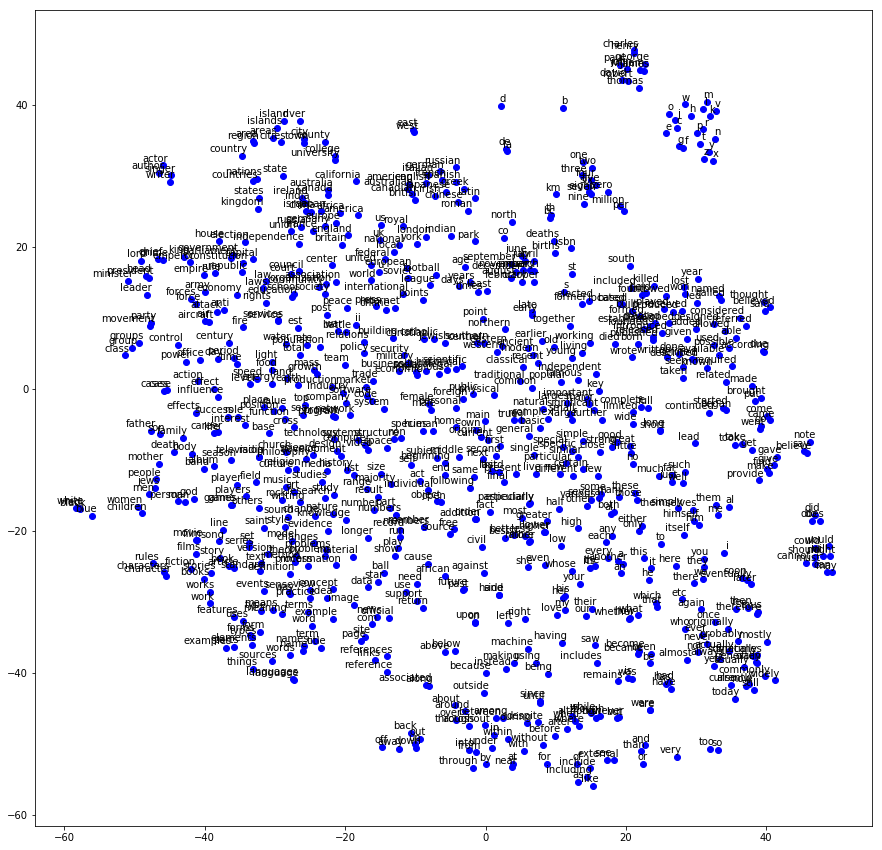
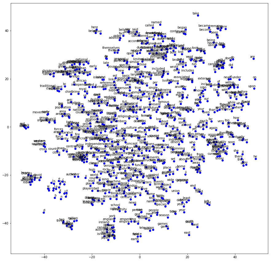
如此一來你將可以簡單的看出,哪些詞彙彼此相似而靠近。
實作CBOW (Continuous Bag of Words)
接著看CBOW的方法,如果我預期輸出的字是target word,從target word向前向後看出去context_window的大小,看到的字都當作我的輸入,所以我輸入的字總共需要context_window*2個,一個target word只會產生一筆數據,如果我一個batch需要batch_size筆數據,我就必須有batch_size個target word,依照這樣的規則下面建立一個Generator來掃描文本,並輸出要訓練使用的Batch Data。
 1
 2
 3
 4
 5
 6
 7
 8
 9
10
11
12
13
14
15
16
17
18
19
20
21
22
23
24
25
26
27
28
29
30
31
32
33
34
35
36
37
38
39
40
41
42
43
44
45
46
47
48
49
50
51
52
53
54
55
56
57
58
59
60
61 | def cbow_batch_generator(data, batch_size, context_window):
span = 2 * context_window + 1 # [ context_window target context_window ]
num_bow = span - 1
batch = np.ndarray(shape=(batch_size, num_bow), dtype=np.int32)
labels = np.ndarray(shape=(batch_size, 1), dtype=np.int32)
buffer = collections.deque(maxlen=span)
# initialization
data_index = 0
for _ in range(span):
buffer.append(data[data_index])
data_index = (data_index + 1) % len(data)
# generate
k = 0
target = context_window
while True:
bow = list(buffer)
del bow[target]
for i, w in enumerate(bow):
batch[k, i] = w
labels[k, 0] = buffer[target]
k += 1
# Recycle
if data_index == len(data):
data_index = 0
# scan data
buffer.append(data[data_index])
data_index = (data_index + 1) % len(data)
# Enough num to output
if k == batch_size:
k = 0
yield (batch, labels)
# demonstrate generator
print('data:', [reverse_dictionary[di] for di in data[:10]])
for context_window in [1, 2]:
batch_generator = cbow_batch_generator(
data=data,
batch_size=8,
context_window=context_window
)
batch, labels = next(batch_generator)
print('\nwith context_window = %d:' % (context_window))
print('batch:')
show_batch = []
for i in range(batch.shape[0]):
tmp = []
for j in range(batch.shape[1]):
tmp.append(reverse_dictionary[batch[i, j]])
show_batch.append(tmp)
print(show_batch)
print('labels:', [reverse_dictionary[li] for li in labels.reshape(8)])
|
| data: ['anarchism', 'originated', 'as', 'a', 'term', 'of', 'abuse', 'first', 'used', 'against']
with context_window = 1:
batch:
[['anarchism', 'as'], ['originated', 'a'], ['as', 'term'], ['a', 'of'], ['term', 'abuse'], ['of', 'first'], ['abuse', 'used'], ['first', 'against']]
labels: ['originated', 'as', 'a', 'term', 'of', 'abuse', 'first', 'used']
with context_window = 2:
batch:
[['anarchism', 'originated', 'a', 'term'], ['originated', 'as', 'term', 'of'], ['as', 'a', 'of', 'abuse'], ['a', 'term', 'abuse', 'first'], ['term', 'of', 'first', 'used'], ['of', 'abuse', 'used', 'against'], ['abuse', 'first', 'against', 'early'], ['first', 'used', 'early', 'working']]
labels: ['as', 'a', 'term', 'of', 'abuse', 'first', 'used', 'against']
|
1
2
3
4
5
6
7
8
9
10
11
12
13
14
15
16
17
18
19
20
21
22
23
24
25
26
27
28
29
30
31
32
33
34
35
36
37
38
39
40
41
42
43
44
45
46
47
48
49
50
51
52
53
54
55
56
57
58
59
60
61
62
63
64
65
66
67
68
69
70
71
72
73
74
75
76
77
78
79
80
81
82
83
84
85
86
87
88
89
90
91
92
93
94
95
96
97
98
99
100
101
102
103
104
105
106
107
108
109
110
111
112
113
114
115
116
117
118
119
120
121
122
123 | class CBOW:
def __init__(self, n_vocabulary, n_embedding,
context_window, reverse_dictionary, learning_rate=1.0):
self.n_vocabulary = n_vocabulary
self.n_embedding = n_embedding
self.context_window = context_window
self.reverse_dictionary = reverse_dictionary
self.weights = None
self.biases = None
self.graph = tf.Graph() # initialize new grap
self.build(learning_rate) # building graph
self.sess = tf.Session(graph=self.graph) # create session by the graph
def build(self, learning_rate):
with self.graph.as_default():
### Input
self.train_dataset = tf.placeholder(tf.int32, shape=[None, self.context_window*2])
self.train_labels = tf.placeholder(tf.int32, shape=[None, 1])
### Optimalization
# build neurel network structure and get their predictions and loss
self.loss = self.structure(
dataset=self.train_dataset,
labels=self.train_labels,
)
# normalize embeddings
self.norm = tf.sqrt(
tf.reduce_sum(
tf.square(self.weights['embeddings']), 1, keep_dims=True))
self.normalized_embeddings = self.weights['embeddings'] / self.norm
# define training operation
self.optimizer = tf.train.AdagradOptimizer(learning_rate=learning_rate)
self.train_op = self.optimizer.minimize(self.loss)
### Prediction
self.new_dataset = tf.placeholder(tf.int32, shape=[None])
self.new_labels = tf.placeholder(tf.int32, shape=[None, 1])
# similarity
self.new_embed = tf.nn.embedding_lookup(
self.normalized_embeddings, self.new_dataset)
self.new_similarity = tf.matmul(self.new_embed,
tf.transpose(self.normalized_embeddings))
### Initialization
self.init_op = tf.global_variables_initializer()
def structure(self, dataset, labels):
### Variable
if (not self.weights) and (not self.biases):
self.weights = {
'embeddings': tf.Variable(
tf.random_uniform([self.n_vocabulary, self.n_embedding],
-1.0, 1.0)),
'softmax': tf.Variable(
tf.truncated_normal([self.n_vocabulary, self.n_embedding],
stddev=1.0 / math.sqrt(self.n_embedding)))
}
self.biases = {
'softmax': tf.Variable(tf.zeros([self.n_vocabulary]))
}
### Structure
# Look up embeddings for inputs.
embed_bow = tf.nn.embedding_lookup(self.weights['embeddings'], dataset)
embed = tf.reduce_mean(embed_bow, axis=1)
# Compute the softmax loss, using a sample of the negative labels each time.
num_softmax_sampled = 64
loss = tf.reduce_mean(
tf.nn.sampled_softmax_loss(weights=self.weights['softmax'],
biases=self.biases['softmax'],
inputs=embed,
labels=labels,
num_sampled=num_softmax_sampled,
num_classes=self.n_vocabulary))
return loss
def initialize(self):
self.weights = None
self.biases = None
self.sess.run(self.init_op)
def online_fit(self, X, Y):
feed_dict = {self.train_dataset: X,
self.train_labels: Y}
_, loss = self.sess.run([self.train_op, self.loss], feed_dict=feed_dict)
return loss
def nearest_words(self, X, top_nearest):
similarity = self.sess.run(self.new_similarity, feed_dict={self.new_dataset: X})
X_size = X.shape[0]
valid_words = []
nearests = []
for i in range(X_size):
valid_word = self.find_word(X[i])
valid_words.append(valid_word)
# select highest similarity word
nearest = (-similarity[i, :]).argsort()[1:top_nearest+1]
nearests.append(list(map(lambda x: self.find_word(x), nearest)))
return (valid_words, np.array(nearests))
def evaluate(self, X, Y):
return self.sess.run(self.new_loss, feed_dict={self.new_dataset: X,
self.new_labels: Y})
def embedding_matrix(self):
return self.sess.run(self.normalized_embeddings)
def find_word(self, index):
return self.reverse_dictionary[index]
|
 1
 2
 3
 4
 5
 6
 7
 8
 9
10
11
12
13
14
15
16
17
18
19
20
21
22
23
24
25
26
27
28
29
30
31
32
33
34 | context_window = 1
# build CBOW batch generator
batch_generator = cbow_batch_generator(
data=data,
batch_size=128,
context_window=context_window
)
# build CBOW model
model_CBOW = CBOW(
n_vocabulary=VOCABULARY_SIZE,
n_embedding=100,
context_window=context_window,
reverse_dictionary=reverse_dictionary,
learning_rate=1.0
)
# initialize model
model_CBOW.initialize()
# online training
epochs = 50
num_batchs_in_epoch = 5000
for epoch in range(epochs):
start_time = time.time()
avg_loss = 0
for _ in range(num_batchs_in_epoch):
batch, labels = next(batch_generator)
loss = model_CBOW.online_fit(X=batch, Y=labels)
avg_loss += loss
avg_loss = avg_loss / num_batchs_in_epoch
print('Epoch %d/%d: %ds loss = %9.4f' % ( epoch+1, epochs, time.time()-start_time, avg_loss ))
|
 1
 2
 3
 4
 5
 6
 7
 8
 9
10
11
12
13
14
15
16
17
18
19
20
21
22
23
24
25
26
27
28
29
30
31
32
33
34
35
36
37
38
39
40
41
42
43
44
45
46
47
48
49
50 | Epoch 1/50: 15s loss = 3.8700
Epoch 2/50: 15s loss = 3.2961
Epoch 3/50: 15s loss = 3.1988
Epoch 4/50: 15s loss = 3.1201
Epoch 5/50: 15s loss = 3.0734
Epoch 6/50: 15s loss = 3.0239
Epoch 7/50: 15s loss = 2.9378
Epoch 8/50: 15s loss = 2.9549
Epoch 9/50: 15s loss = 2.9651
Epoch 10/50: 15s loss = 2.9028
Epoch 11/50: 15s loss = 2.8770
Epoch 12/50: 15s loss = 2.8298
Epoch 13/50: 15s loss = 2.8437
Epoch 14/50: 15s loss = 2.7681
Epoch 15/50: 15s loss = 2.7823
Epoch 16/50: 15s loss = 2.7867
Epoch 17/50: 15s loss = 2.7540
Epoch 18/50: 15s loss = 2.7567
Epoch 19/50: 15s loss = 2.7340
Epoch 20/50: 15s loss = 2.6212
Epoch 21/50: 15s loss = 2.5187
Epoch 22/50: 15s loss = 2.7150
Epoch 23/50: 15s loss = 2.6647
Epoch 24/50: 15s loss = 2.7381
Epoch 25/50: 15s loss = 2.5337
Epoch 26/50: 15s loss = 2.6587
Epoch 27/50: 15s loss = 2.6648
Epoch 28/50: 15s loss = 2.5963
Epoch 29/50: 15s loss = 2.5418
Epoch 30/50: 15s loss = 2.6041
Epoch 31/50: 15s loss = 2.5535
Epoch 32/50: 15s loss = 2.5928
Epoch 33/50: 15s loss = 2.5535
Epoch 34/50: 15s loss = 2.5233
Epoch 35/50: 15s loss = 2.5658
Epoch 36/50: 15s loss = 2.5966
Epoch 37/50: 15s loss = 2.5422
Epoch 38/50: 15s loss = 2.5673
Epoch 39/50: 15s loss = 2.5142
Epoch 40/50: 15s loss = 2.5175
Epoch 41/50: 15s loss = 2.4909
Epoch 42/50: 15s loss = 2.4872
Epoch 43/50: 15s loss = 2.5513
Epoch 44/50: 15s loss = 2.4917
Epoch 45/50: 15s loss = 2.5198
Epoch 46/50: 15s loss = 2.5007
Epoch 47/50: 15s loss = 2.2530
Epoch 48/50: 15s loss = 2.4154
Epoch 49/50: 15s loss = 2.4927
Epoch 50/50: 15s loss = 2.4948
|
| valid_words_index = np.array([10, 20, 30, 40, 50, 210, 239, 392, 396])
valid_words, nearests = model_CBOW.nearest_words(X=valid_words_index, top_nearest=8)
for i in range(len(valid_words)):
print('Nearest to \'{}\': '.format(valid_words[i]), nearests[i])
|
 1
 2
 3
 4
 5
 6
 7
 8
 9
10
11
12 | Nearest to 'two': ['three' 'four' 'five' 'six' 'seven' 'eight' 'nine' 'zero']
Nearest to 'that': ['which' 'what' 'furthermore' 'however' 'talmudic' 'endress' 'tonight'
'how']
Nearest to 'his': ['her' 'their' 'my' 'your' 'its' 'our' 'the' 'photographs']
Nearest to 'were': ['are' 'have' 'include' 'contain' 'was' 'vigorous' 'tend' 'substituting']
Nearest to 'all': ['various' 'both' 'many' 'every' 'shamed' 'everyone' 'those' 'wiccan']
Nearest to 'area': ['areas' 'region' 'regions' 'taipan' 'northeast' 'boundaries' 'hattin'
'surface']
Nearest to 'east': ['west' 'southeast' 'south' 'northwest' 'southwest' 'eastern' 'northeast'
'north']
Nearest to 'himself': ['him' 'themselves' 'herself' 'itself' 'them' 'donal' 'activex' 'carnaval']
Nearest to 'white': ['black' 'red' 'morel' 'green' 'bluish' 'dead' 'blue' 'lessig']
|
1
2
3
4
5
6
7
8
9
10
11
12
13
14
15
16
17
18
19
20
21
22 | from matplotlib import pylab
from sklearn.manifold import TSNE
def plot(embeddings, labels):
assert embeddings.shape[0] >= len(labels), 'More labels than embeddings'
pylab.figure(figsize=(15, 15)) # in inches
for i, label in enumerate(labels):
x, y = embeddings[i, :]
pylab.scatter(x, y, color='blue')
pylab.annotate(label, xy=(x, y), xytext=(5, 2), textcoords='offset points',
ha='right', va='bottom')
pylab.show()
visualization_words = 800
# transform embeddings to 2D by t-SNE
embed = model_CBOW.embedding_matrix()[1:visualization_words+1, :]
tsne = TSNE(perplexity=30, n_components=2, init='pca', n_iter=5000, method='exact')
two_d_embed = tsne.fit_transform(embed)
# list labels
words = [model_CBOW.reverse_dictionary[i] for i in range(1, visualization_words+1)]
# plot
plot(two_d_embed, words)
|
Reference
- https://github.com/tensorflow/tensorflow/blob/master/tensorflow/examples/udacity/5_word2vec.ipynb